solve_ivp from the ground up: the pendulum beyond small angles

Afterwards you can integrate any system of first-order ODEs with solve_ivp, control its accuracy, and pull events such as zero crossings out of the solution.

Topic: Ordinary differential equations
Field: Mathematics, Physics
Libraries: matplotlib 3.11.2, numpy 2.5.3, scipy 1.18.1
Prerequisites: none beyond Python basics
Notebook: Download py-solve-ivp.ipynb, executed with the versions above

The problem: how long does a pendulum swing?

Every textbook gives the period of a pendulum as \(T_0 = 2\pi\sqrt{L/g}\). For a 1 m pendulum that is 2.006 s. The textbook also says, usually in smaller print, that this holds for small angles only. How wrong is it at 30°? At 90°? At 170°, where you have pulled the bob almost up to the top?

The equation of motion is

\[\ddot\theta = -\frac{g}{L}\sin\theta ,\]

and the trouble is the sine. Replace it by \(\theta\) and you get the harmonic oscillator and the formula above. Keep it and there is no elementary solution. There is an exact answer in terms of an elliptic integral, and we will use it at the end to check our work, but the numerical route is the one you will take for every other equation you meet, because almost none of them has an exact answer.

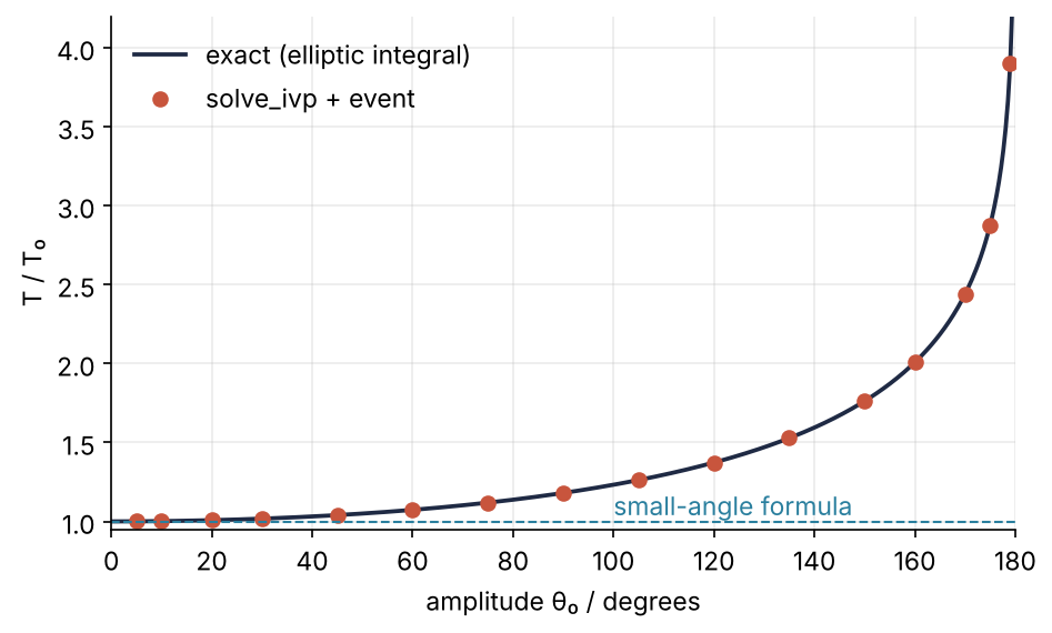
Period of a pendulum relative to the small-angle value, as a function of amplitude. Dots: solve_ivp. Line: exact elliptic integral.

This is where we end up: the period rises slowly at first, is 18 % too long at 90°, and runs away as the amplitude approaches 180°. Each dot is one call to solve_ivp plus one event detection. The rest of this tutorial builds that figure.

Setup

import numpy as np
import matplotlib.pyplot as plt
from scipy.integrate import solve_ivp

g = 9.81   # m/s^2
L = 1.0    # m
T0 = 2 * np.pi * np.sqrt(L / g)

plt.rcParams.update({
    "figure.figsize": (7, 3.6), "figure.dpi": 110,
    "axes.spines.top": False, "axes.spines.right": False,
    "axes.grid": True, "grid.alpha": 0.25,
    "font.size": 11, "lines.linewidth": 1.8,
})
INK, ACCENT, SECOND = "#1f2a44", "#c8553d", "#2a7f9e"

print(f"small-angle period T0 = {T0:.4f} s")

small-angle period T0 = 2.0061 s

Step 1: Write the equation the way solve_ivp wants it

solve_ivp solves first-order systems \(\dot{\mathbf y} = \mathbf f(t, \mathbf y)\). A second-order equation becomes two first-order ones by introducing the angular velocity \(\omega = \dot\theta\):

\[\dot\theta = \omega, \qquad \dot\omega = -\frac{g}{L}\sin\theta .\]

The state vector is \(\mathbf y = (\theta, \omega)\), and the right-hand side is a plain function that takes the time and the state and returns the derivatives, in the same order:

def pendulum(t, y):
    theta, omega = y
    return [omega, -(g / L) * np.sin(theta)]

Three things to get right. The time comes first in the signature, even though this equation does not use it. The function receives the whole state as one array and returns the whole derivative as one list or array of the same length. And you return the derivatives, not the new state. solve_ivp does the stepping; you only tell it the slope.

Step 2: Call it and look at what comes back

Release the pendulum from rest at 90° and integrate for ten seconds:

theta0 = np.radians(90)
sol = solve_ivp(pendulum, (0, 10), [theta0, 0.0])
print(sol)

  message: The solver successfully reached the end of the integration interval.
  success: True
   status: 0
        t: [ 0.000e+00  1.019e-04 ...  9.673e+00  1.000e+01]
        y: [[ 1.571e+00  1.571e+00 ...  1.340e+00  2.219e-01]
            [ 0.000e+00 -9.994e-04 ... -2.089e+00 -4.361e+00]]
      sol: None
 t_events: None
 y_events: None
     nfev: 254
     njev: 0
      nlu: 0

The result is a bunch of fields. sol.t holds the times at which the solver stopped, sol.y the states at those times, one row per component. So sol.y[0] is \(\theta(t)\) and sol.y[1] is \(\omega(t)\). status 0 and success True mean it reached the end. nfev is the number of times your function was called, a useful cost meter later on.

Look at the times:

print(sol.t.shape, sol.y.shape)
with np.printoptions(precision=4, suppress=True):
    print(sol.t[:8])

(33,) (2, 33)
[0.     0.0001 0.0011 0.0113 0.1132 0.6012 0.8939 1.1866]

Only 33 points for ten seconds, and they are not evenly spaced. The solver takes tiny steps at the start, while it is still measuring how fast the solution changes, then settles into steps of about a third of a second. Plot it with markers and you see the grid:

fig, ax = plt.subplots()
ax.plot(sol.t, np.degrees(sol.y[0]), "o-", color=INK, ms=4)
ax.set(xlabel="t / s", ylabel="θ / degrees")
plt.show()

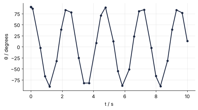
The curve looks angular because the solver did not stop anywhere between its steps. It did not need to: its internal accuracy is fine. It just did not store anything in between.

Step 3: Get the solution where you want it

For a smooth plot you want the solution on your own grid. Two ways. t_eval asks for output at given times:

t = np.linspace(0, 10, 500)
sol = solve_ivp(pendulum, (0, 10), [theta0, 0.0], t_eval=t)
print(sol.y.shape, "nfev =", sol.nfev)

(2, 500) nfev = 254

dense_output=True returns a function you can evaluate anywhere afterwards:

sol = solve_ivp(pendulum, (0, 10), [theta0, 0.0], dense_output=True)
theta_at = lambda t: sol.sol(t)[0]
print(np.degrees(theta_at([0.5, 1.0, 1.5])))

[ 23.06975114 -80.52757451 -62.05530818]

Note that nfev is 254 in both cases, exactly as in Step 2. Neither option changes the steps the solver takes. It interpolates between them, with an interpolant that matches the accuracy of the method. Which raises the question what that accuracy is.

Step 4: Control the accuracy

The two knobs are rtol and atol. At every step the solver keeps the estimated error of each component below atol + rtol * |y|. The defaults are rtol=1e-3 and atol=1e-6, and the first of these is loose: three significant digits.

For the pendulum there is a sharp test. Energy is conserved, so

\[E = \tfrac12 L^2\omega^2 + gL(1-\cos\theta)\]

must stay constant. Integrate for 100 s, about fifty swings, and watch how much it drifts:

def energy(y):
    theta, omega = y
    return 0.5 * L**2 * omega**2 + g * L * (1 - np.cos(theta))

for rtol, atol in [(1e-3, 1e-6), (1e-6, 1e-9), (1e-10, 1e-12)]:
    s = solve_ivp(pendulum, (0, 100), [theta0, 0.0], rtol=rtol, atol=atol)
    E = energy(s.y)
    drift = np.max(np.abs(E - E[0])) / E[0]
    print(f"rtol={rtol:<6g} atol={atol:<6g} nfev={s.nfev:6d}  max energy drift {drift:.1e}")

rtol=0.001  atol=1e-06  nfev=  2360  max energy drift 8.6e-02

rtol=1e-06  atol=1e-09  nfev=  8630  max energy drift 7.4e-05

rtol=1e-10  atol=1e-12  nfev= 44108  max energy drift 1.1e-08

With the defaults the energy wanders by 9 %. The pendulum you integrated is not the pendulum you wrote down. Tightening to 1e-6 costs four times as many evaluations and brings the drift to a hundredth of a percent; 1e-10 costs twenty times and gives eight digits. On a two-component system this is still milliseconds, so the rule is simple: never trust the defaults for anything you will plot, measure, or publish. Set rtol=1e-8, atol=1e-10 and only loosen it when the run time actually hurts.

Step 5: Find the period with an event

The period is the time between two successive passages through \(\theta = 0\) in the same direction. You could search sol.y[0] for sign changes and interpolate, but solve_ivp does this for you, to full accuracy, through events. An event is a function of \((t, \mathbf y)\) whose zero the solver locates:

def upward_crossing(t, y):
    return y[0]                   # zero when theta = 0

upward_crossing.direction = 1     # only count crossings from negative to positive

sol = solve_ivp(pendulum, (0, 20), [theta0, 0.0],
                events=upward_crossing, rtol=1e-8, atol=1e-10)
crossings = sol.t_events[0]
print(np.round(crossings, 4))
print("periods:", np.round(np.diff(crossings), 6))

[ 1.7759  4.1437  6.5116  8.8794 11.2472 13.6151 15.9829 18.3508]
periods: [2.367842 2.367842 2.367842 2.367842 2.367842 2.367842 2.367842]

Seven periods, all 2.367842 s, constant to the sixth digit. The direction attribute matters: without it you count downward crossings too and get half-periods. Setting terminal = True on the event would stop the integration at the first hit, which is what you want when a projectile reaches the ground.

Now the check against the exact result. The period of the pendulum is \(T = 4\sqrt{L/g}\,K(k^2)\) with \(k = \sin(\theta_0/2)\) and \(K\) the complete elliptic integral of the first kind, which SciPy provides as scipy.special.ellipk:

from scipy.special import ellipk

T_num = np.diff(crossings).mean()
T_exact = 4 * np.sqrt(L / g) * ellipk(np.sin(theta0 / 2) ** 2)
print(f"numeric {T_num:.7f} s   exact {T_exact:.7f} s   T/T0 = {T_exact / T0:.4f}")

numeric 2.3678419 s   exact 2.3678419 s   T/T0 = 1.1803

Seven digits of agreement, and the answer to the opening question: at 90° the textbook formula is 18 % short.

Step 6: Sweep the amplitude

Wrap Step 5 in a function and call it for amplitudes from 5° to 179°. Starting from rest at \(\theta_0\), the solver needs a few periods to collect crossings, and the period near 180° is four times \(T_0\), so the integration window has to grow with the amplitude:

def period(theta0_deg):
    th0 = np.radians(theta0_deg)
    s = solve_ivp(pendulum, (0, 12 * T0), [th0, 0.0],
                  events=upward_crossing, rtol=1e-8, atol=1e-10)
    return np.diff(s.t_events[0]).mean()

amplitudes = np.array([5, 10, 20, 30, 45, 60, 75, 90, 105, 120, 135, 150, 160, 170, 175, 179])
T_num = np.array([period(a) for a in amplitudes])

a_fine = np.linspace(0, 179.9, 400)
T_exact = 4 * np.sqrt(L / g) * ellipk(np.sin(np.radians(a_fine) / 2) ** 2)

fig, ax = plt.subplots(figsize=(7, 4))
ax.plot(a_fine, T_exact / T0, color=INK, label="exact (elliptic integral)")
ax.plot(amplitudes, T_num / T0, "o", color=ACCENT, ms=6, label="solve_ivp + event")
ax.axhline(1, color=SECOND, lw=1, ls="--")
ax.text(100, 1.04, "small-angle formula", color=SECOND)
ax.set(xlabel="amplitude θ₀ / degrees", ylabel="T / T₀", xlim=(0, 180), ylim=(0.95, 4.2))
ax.legend(frameon=False, loc="upper left")
plt.show()

for a, T in zip(amplitudes[::3], T_num[::3]):
    print(f"{a:4d}°   T/T0 = {T / T0:.4f}")

   5°   T/T0 = 1.0005
  30°   T/T0 = 1.0174
  75°   T/T0 = 1.1190
 120°   T/T0 = 1.3729
 160°   T/T0 = 2.0075
 179°   T/T0 = 3.9010

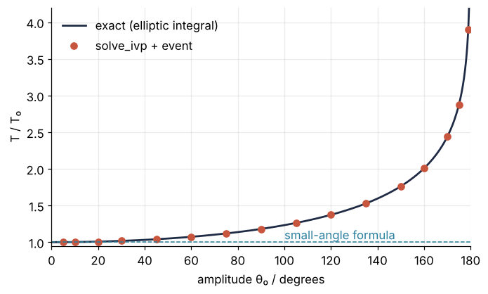
At 30° the textbook formula is off by under 2 %, which is why it survives in textbooks. At 75° it is 12 % short, at 120° 37 %, and at 160° the pendulum takes twice as long as the formula says. The dots sit on the exact curve to better than the marker size. Sixteen amplitudes took sixteen solver calls and well under a second.

Pitfalls

Passing parameters the wrong way. If your right-hand side takes extra arguments, say def pendulum(t, y, g, L), hand them over with args=(g, L). The common mistake is args=g for a single parameter; args must be a tuple, so write args=(g,) with the trailing comma. The error message, something like pendulum() argument after * must be an iterable, does not say so.

Mixing up the axes of sol.y. sol.y has shape (n_components, n_times). sol.y[0] is the first component over all times, sol.y[:, 0] is the full state at the first time. If you plot sol.y directly you get one line per time step instead of one per component, and for 500 steps the figure is a wall of lines. When in doubt, sol.y.T gives the layout most people expect.

Using the default method on a stiff problem. Some equations contain processes on wildly different time scales, a fast one that decays quickly and a slow one you care about. The default RK45 then has to take steps dictated by the fast process even after it has died away. The Van der Pol oscillator with a large damping parameter is the standard example:

def vdp(t, y, mu):
    x, v = y
    return [v, mu * (1 - x**2) * v - x]

for method in ["RK45", "Radau"]:
    s = solve_ivp(vdp, (0, 500), [2.0, 0.0], method=method, args=(200,), rtol=1e-6, atol=1e-9)
    print(f"{method:6s} nfev = {s.nfev:7d}")

RK45   nfev =  387482

Radau  nfev =    9005

A factor of forty in function evaluations, for a two-component system. If nfev runs into the hundreds of thousands, or the solver seems to hang, switch to method="Radau" or "LSODA". They are built for this.

Variations

Damped and driven. Add \(-\gamma\omega + A\cos(\Omega t)\) to the second component and pass \(\gamma, A, \Omega\) through args. For \(A\) around 1.2 and \(\Omega = 2/3\) in units where \(g/L = 1\), the motion is chaotic, and dense_output is what you need to build a Poincaré section.
Projectile with air drag. State \((x, y, v_x, v_y)\), drag proportional to \(v^2\), and an event y = 0 with terminal = True and direction = -1 that stops the integration on impact. sol.y_events[0] then holds the landing state.
The double pendulum. Four components, and the right-hand side is a page of algebra. Everything in this tutorial carries over unchanged; only the energy check becomes mandatory, because the equations are easy to get wrong.
An epidemic. The SIR model has three components and a parameter pair \((\beta, \gamma)\). An event on \(\dot I = 0\) finds the peak of the epidemic without any post-processing.

Cheat sheet

sol = solve_ivp(f, (t0, t1), y0,
                args=(p1, p2),              # extra arguments of f(t, y, p1, p2); tuple!
                rtol=1e-8, atol=1e-10,      # defaults 1e-3 / 1e-6 are too loose
                t_eval=t,                   # output at these times
                dense_output=True,          # sol.sol(t) evaluates anywhere
                events=[ev1, ev2],          # ev(t, y) = 0 is located; ev.direction, ev.terminal
                method="RK45")              # "Radau" or "LSODA" for stiff problems
sol.t, sol.y[i]                             # times, i-th component over time
sol.t_events[k], sol.y_events[k]            # times and states where event k fired
sol.status, sol.message, sol.nfev           # 0 = reached t1; cost meter